This is a comprehensive review of everything I learned following Stanford's CS231n and completing assignment 1. For resources I used the CS231n lectures and notes (until the lectures were taken down) and I occasionally used this forum. I was also assisted by a professor from my school who helped walk me through some of the more complex topics.
My goal in completing this assignment was to have a good understanding of the fundamental concepts behind neural networks and deep learning. I admit, I did make this course more challenging for myself as I had no understanding of linear algebra or multivariable calculus (both pre-reqs) prior to taking this course; however, in retrospect, with the aid of the course notes, lecture videos, my teacher and the forum, I was able to implement a lot of the code myself.
I am writing this blog post because I feel it is both a good way to take notes to look back on in the future, and a strong way to prove to myself that I really do have a solid understanding of the material.
Introduction
Computer Vision
One particularly relevant application of deep learning and neural networks to this course is computer vision. Understanding how to give computers the benefit of sight has been a key goal in the computer science community that came about in the very early days of vision. As researchers found, understanding computer vision is as much about understanding computers as it is about understanding human vision as that is inevitably what is trying to be replicated. Over the past fifty years, our understanding of human vision has shifted from a holistic approach to an hierarchical approach. Previously it was thought that the brain would store whole objects in a very specific part of the brain, now, with the hierarchical approach, it is believed that vision can be broken down into much smaller components then objects. Edges, for instance, are believed to define shapes so instead of storing an object somewhere in our brains we store a set of edges and lines that make up that object and only upon the triggering of those very specific edges and lines do we understand what an object is. With these specific edges and lines, humans are able to build complex 3d representations of objects within our head, which allows us to understand what objects are no matter their orientation, color, etc. The overarching goal is to build this 3d model of objects within the computer.
The first approach to solving vision was edge detection and then moved into segmentation for feature detection. An example of this would be detecting for specific shapes in an image, say the straight legs of a chair a certain distance apart. For almost sixty years, people attempted unsuccessfully to solve vision using this method. Now focus has shifted to deep learning as it has achieved promising results over the past couple years in the field of machine learning. This isn't to say that Deep Learning hadn't existed until recently, as the first neural networks were built in the 60's, but it is to say that very few focused on it as a solution because it was just too slow and computationally costly.
Image Classification
Image classification means taking an image and transforming it into one of a fixed number of categories. This is easier said than done because of a number of environment variables like rotation, point of view, illumination, deformation, occlusion, background clutter and interclass variation. Over the past sixty years two approaches have been taken: the explicit approach and the data driven approach. An example of an explicit approach is feature detection (the search for two straight lines a certain distance from each other to classify a chair). The issue with this approach is that every time you want to classify a new object a new algorithm must be hard coded to look for certain characteristics, making this method incapable of major growth. Deep learning follows the latter approach, which involves collecting a very large dataset of images and labels and then training algorithms using machine learning.
Assignment 1
In this assignment I will implement the k-nearest neighbor classifier, a support vector machine, the softmax classifier, backpropagation (stochastic gradient descent) and a neural net.
K-Nearest Neighbor Classifier
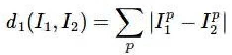
This classifier literally compares an image for similarities to a dataset. After finding the most similar image/images in the dataset, it classifies the original image with the class of the similar image/images. By similar I am referring to the distances between the two images. Two different methods can be used to find the distance, the L1/Manhattan distance:
And the L2/Euclidean distance:
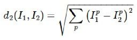
The image with the smallest distance between the two is considered to be the most similar image. This is called the nearest neighbor classifier. The K-nearest neighbor classifier is very similar as instead of selecting just one most similar images, it selects K most similar images and then classifies the image based off the class that has the majority in the K images.
In this particular assignment we were asked to implement this classifier using the Euclidean/L2 distance in three different ways: with two for loops, with one for loop and with no for loops. This is designed to introduce us to vectorizing code.
Two Loops
First I just convert the equation for Euclidean distance into numpy operation:
num_test = X.shape[0]
num_train = self.X_train.shape[0]
dists = np.zeros((num_test, num_train))
for i in xrange(num_test):
    for j in xrange(num_train):
        dists[i,j] = np.sqrt(np.sum(np.square(X[i]-self.X_train[j])))
return dists
Where X[i] is the image we are attempting to find the class for and X_train[j] is the remainder of the images in the training set.
One Loop
Reducing the same operation to one loop:
for i in xrange(num_test):
    dists[i,:] = np.sqrt(np.sum(np.square(X[i,:]-self.X_train),axis =1))
return dists
The important thing to understand in this case is what exactly something like dists[i,:] is doing. From playing around with it and from the python tutorial, I figured out that his would represent every column in row i. It is just a more efficient way to compare every picture to the dataset.
No Loops
Now we take it a step further, computing the Euclidean distance without loops:
dists = np.sqrt((X**2).sum(axis=1)[:, np.newaxis] + (self.X_train**2).sum(axis=1) - 2 * X.dot(self.X_train.T))
return dists
To put this into perspective I will do it on a much simpler scale. Instead of dealing with these huge matrices, pretend we are just working with two vectors, q and p. To find the Euclidean distance between these two vectors we find the length of its distance vector:

Otherwise written as:

Alright, now that we understand how to find the length of the two vector's distance vector, the same process is applied to the bigger matrices.
Linear Classifier
Although this is not a direct part of the assignment, it is necessary to understand what exactly the Support Vector Machine and the Softmax classifier are doing. A linear classifier involves an input(an image in this case) and a set of initially arbitrary parameters known as weights. Here it is in its most basic form:
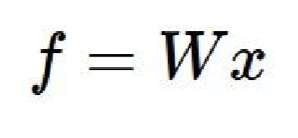
Where x is the image's pixels (stretched into rows) and W is a matrix with as many rows as there are dimensions in the images and as many columns as there are classes. When the two are multiplied together we get a score for each class. Basically we are computing a weighted sum of all the pixel values for each score. Ideally when we pass an image through, the correct classifier will have the highest score; however, this is often not the case which is where the SVM and the Softmax classifier come in. These classifiers are used to interpret the scores and quantify how poorly our linear classifier is working. can be used It is important to note that the scores will be score free, and when first training a linear classifier, selected at random.
Support Vector Machine
Using the output of a linear classifier given random weights, the intent of the SVM is to gauge the degree of how wrong the classification is. It does this by repeatedly finding the difference between the lowest score and the correct score for each image. With the output we can identify how to change the linear classifiers weights in order to improve classification on its next pass. That was a very high level overview, now to look at exactly what is happening:
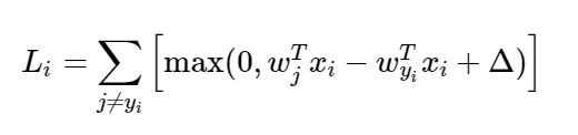
Where Li is the loss for a single training example, x is a vector of images, w is a vector of weights, y is a vector of labels and delta represents the safety margin. The max is taken in order to clamp possible loss at zero so negative numbers will not have a bearing on the overall loss of the function. If negative loss was allowed to pass through, it would decrease the overall loss which can distort the overall loss and make it seem like we are closer to identifying the correct scores even if we aren't. For the overall loss we must average the loss over all the images:
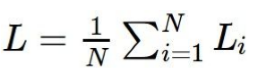
Where N is the number of training examples.
In this part of the assignment we first compute the loss and the gradient with loops before implementing a vectorized version.
With Loops:
First off, I need to refer you to the course notes as it goes through many aspects of this part of the assignment. Naturally it is a good idea to start by implementing the SVM loss function. After I implemented the loss function I also implemented something called the regularization loss:
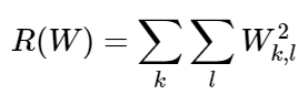
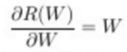
Regularization of the Weights(W).
As the notes explain, regularization is important because often times there will be multiple sets of weights that will correctly classify the images. However, it is important to not be optimizing for all of them and instead be optimizing for only one set of weights. This is where regularization comes in. All regularization does is discourage large weights by using an "elementwise quadratic penalty". We then incorporate this into the loss function along with some hyper parameter lamda which controls how much effect the regularization loss has:
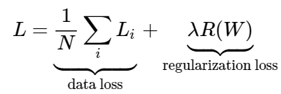
Or fully expanded:
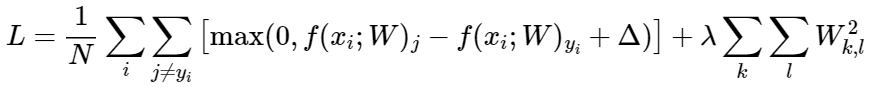
After trying unsuccessfully to get the right gradient, I checked the forum and it actually turns out that the equation they use for regularization loss is:

Now to implement the code:
# compute the loss
num_classes = W.shape[1]  # how many classes
num_train = X.shape[0] # how many images are in the training dataset
loss = 0.0
for i in xrange(num_train):
    scores = X[i].dot(W) #linear classifier
    dT = np.zeros(W.shape) # create an array the same size as the weight matrix made entirely out of zeros
    correct_class_score = scores[y[i]]
    for j in xrange(num_classes):
        if j == y[i]: #importantly the loss is not calculated when you are comparing an image to itself as it would give a value of (delta) which would have a non universal affect on the overall loss.
            continue
        margin = scores[j] - correct_class_score + 1 # note delta = 1
        if margin > 0:
            loss += margin

# finding the overall loss
loss /= num_train


# Add regularization to the loss.
loss += 0.5 * reg * np.sum(W * W)

return loss
Now to include the gradient. As the course notes tell us the equation for the gradient of an SVM can be found by taking the gradient with respect to (wyi). The 1 in this equation is supposed to be an indicator function:
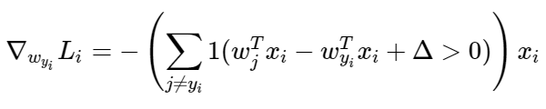
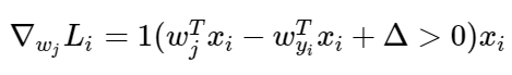
It then goes on to tell us, and I quote, "when you’re implementing this in code you’d simply count the number of classes that didn’t meet the desired margin (and hence contributed to the loss function) and then the data vector (Xi) scaled by this number is the gradient". The equation above is only the gradient with respect to the row of W that "corresponds with the correct class." Where J does not equal yi the gradient is:
Finally, we also must take the gradient of the regularization loss which comes out to:
So we will include the gradient:
# compute the loss and the gradient
num_classes = W.shape[1]
num_train = X.shape[0]
loss = 0.0
for i in xrange(num_train):
    scores = X[i].dot(W)
    dW = np.zeros(W.shape) #initializing the gradient
    correct_class_score = scores[y[i]]
    gradCounter = 0 #keeping track of the number of positive scores
    for j in xrange(num_classes):
        if j == y[i]:
            continue
        margin = scores[j] - correct_class_score + 1
        if margin > 0:
            loss += margin
            dW[:,j] = X[i] #updating the gradient for incorrect rows with the image
            gradCounter += 1
    #adding the gradient to the column of the correct class
    dW[:,y[i]] = -(gradCounter  * X[i])

#regularize the gradient
dW = reg*W
Full gradient:
dW += dW/num_train

# We want the loss to be an average of all the training examples so we divide by num_train
loss = loss/num_train

# Add regularization to the loss.
loss += 0.5 * reg * np.sum(W * W)

return loss, dW
Vectorized
Now for the hard part: vectorizing the equations we just used above. This is one of those cases where I resorted to the forum for understanding after four or five hours of unsuccessful attempts. To be as clear as possible, this is not my code. Although I have partial explanations in the comments, when I have time I plan on putting matrices next to this code for each step to show exactly what is happening.
loss = 0.0
num_train = X.shape[0]
num_classes = W.shape[1]
dW = np.zeros(W.shape) # initialize the gradient as zero


#Vectorized version of the SVM loss
score = X.dot(W) #linear classifier

y_pred = score[range(score.shape[0]),y]

#SVM loss
margins = score - y_pred[:,None] + 1 #
margins[range(score.shape[0]),y] = 0
margins = np.maximum(np.zeros(margins.shape),margins)
loss = np.sum(margins)
loss /= num_train #average loss
loss += 0.5 * reg * np.sum(W*W) #regularization


#Vectorized version of the gradient
Mc = (margins>0).astype(float)
Mc[np.arange(num_train), y] = -1
dW = np.dot(X.T, Mc)/ num_train + reg * W

return loss, dW
Optimization
Through using either the SVM or the Softmax classifier (which I will address later) we can obtain the loss; however, we lack a way of improving the classifier. One method is to randomly increase and decrease the weights and use the weights that yield the smallest loss. Or, as this is terrible method, we could follow the slope.
Numerical Gradient
The numerical gradient is found by taking the slope in a bunch of different directions. Through this we are finding the gradient, or what direction is uphill, however we are trying to decrease our values so we will take the negative of the gradient and take a small step down hill. This method is effective but it is incredibly slow and computationally expensive… it is the reason people focused on feature detection for 50 years. Instead we will predominately use a technique called backpropagation which is much less computationally expensive. However, the numerical gradient is still utilized to perform gradient checks on backpropagation as it is much more reliable.
Analytic Gradient: Backpropagation
To understand backpropagation you have to understand the chain rule with partial derivatives. After that it is rather straightforward as backpropagation is the recursive application of chain rule through a computational graph to find the influence of every intermediate value in the graph on the final loss function. This enables you to find the effects that the inputs have on the output of the loss function. There is an entire section of the course notes which explains this.
Stochastic Gradient Descent
In the SVM part of the assignment, they also ask us to write a few lines of code in the linear classifier file to implement stochastic gradient descent. The course notes inform us that stochastic gradient descent explicitly refers to doing gradient descent (changing the values of the weights in an effort to improve classification accuracy) with only one example. However, stochastic gradient descent is often used to refer to mini-batch gradient descent as well, which trains on multiple examples. Technically we are implementing mini-batch gradient descent here. First they ask us to sample some batch size elements from the training data and the corresponding labels. Further they give us a hint to use the np.random.choice function to generate indices. With all this in mind, it becomes pretty he to do this part.
 z = np.random.choice(num_train, batch_size,replace=True) # take a random batch, size batch_size, from the array num_train
 X_batch = X[z] # retrieve the images and their values
 y_batch = y[z]
Next they ask us to update the weights using the gradient and the learning rate. The learning rate is just another word for step size, this variable adjusts how quickly we are attempting to optimize. We have already done something very similar to this in the SVM implementation:
self.W += -learning_rate * grad
Finally they ask us to implement the predict method to predict the labels for the data points:
y_pred = np.argmax(X.dot(self.W), axis=1) #returns the indices of the maximum value of the interior function, which is just the linear classifier.
Softmax Classifier
Again using the scores outputted from the linear classifier given random weights, the softmax classifier interprets the scores as the unnormalized log probabilities of the classes (Andrej mentioned the reason behind this interpretation is very complex). So we first exponentiate the scores, normalize them and then take the -log to retrieve the probabilities of the classes. We then attempt to maximize the log likelihood and minimize the -log likelihood of the true class. Two sets of course notes that were really helpful to me when I implemented this can be found here and here. Here is an equation for what I just described.
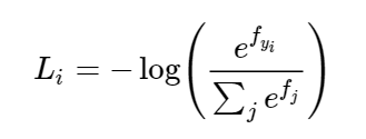
Where Li is the loss for a single example, f is the array of class scores for a single example.
The gradient of which would be:
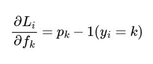
Where P is a vector of the normalized probabilities. The notes also emphasize a point on ensuring numerical stability as we could potentially be dealing with large numbers. They suggest we implement an equation like this:
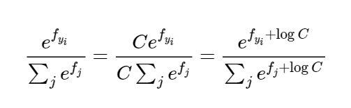
Further, the notes go on to tell us that it is common choice for C is to set:
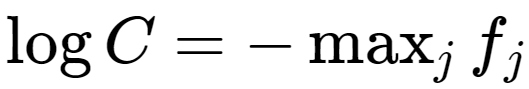
Here is the implementation with loops:
With Loops
#Initialize the loss and gradient to zero.
loss = 0.0
dW = np.zeros(W.shape)

num_classes = W.shape[1]
num_train = X.shape[0]
for i in xrange(num_train):
    scores = X[i].dot(W) #linear classifier
    scores -= np.max(scores)  #numerical stability
    prob = np.exp(scores)/np.sum(np.exp(scores), axis=1, keepdims = True) #exponentiation and normalization
    loss += -np.log(prob[y[i]])  #-log
    for j in xrange(num_classes):
        dW[:,j] += (prob[j]-(j == y[i])) * X[i] #updating the gradient
loss /= num_train #overall loss
loss += 0.5 * reg * np.sum(W * W) #regularization
dW = (1.0/num_train)*dW
dW += reg*W #weight regularization

return loss, dW
###Vectorized
Again I struggled for hours trying to figure out how to do this myself before resorting to the forum. If it is at all unclear, this is not my code; however, I did spend a great deal of time endeavoring to understand the motivation behind every line. Although I have partial explanations in the comments, when I have time I plan on putting matrices next to this code for each step to show exactly what is happening. scores = X.dot(W) # linear classifer scores -= np.max(scores,axis=1).reshape(num_train,1)
#softmax with numerical stability
prob = np.exp(scores)/np.reshape(np.sum(np.exp(scores),axis=1),(num_train,1)
loss = -np.sum(np.log(prob[(range(num_train),y)]))
loss /= num_train
#final loss with weight regularization
loss += 0.5 * reg * np.sum(W * W)

#calculating the gradient w/ weight regularization
prob[(range(num_train),y)] = prob[(range(num_train),y)] - 1
dW = (1.0/num_train) * np.dot(X.T,prob) + reg * W

return loss, dW
Two-Layer Neural Network
Looking at the equation of a neural network is probably the best way to understand what exactly it is. Here's an equation for a 3 layer Neural Network:
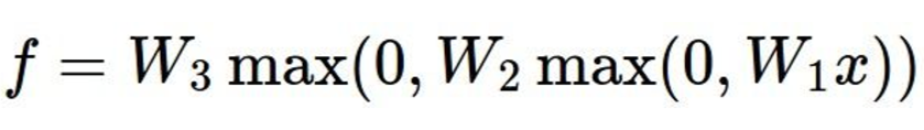
Now a two layer:
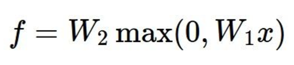
Finally a linear classifier:
It is just a matter of embedding linear classifiers within each other, allowing for multiple sets of weights which means more detail about the image. In this part of the assignment we are asked to implement a two layer neural network.
Forward Pass and Computing the Loss
The first three lines of code are simply executing the equation for the two layer neural net described above.
layer1 = np.dot(X,W1) + b1
layer2 = np.maximum(0,layer1)
scores = np.dot(layer2,W2) + b2
This is just the soft max loss with some minor adjustments as we are dealing with two sets of weights. Notably the hidden layer uses a "ReLU" non-linearity. This function just means to take the maximum of 0 and x.
#softmax loss
scores -= np.max(scores,axis=1)[:,np.newaxis]
prob = np.exp(scores)/np.sum(np.exp(scores),axis=1)[:,np.newaxis]
loss = -np.sum(np.log(prob[(xrange(N),y)]))
loss /= N
loss += 0.5 * reg * np.sum(W1 * W1)
loss += 0.5 * reg * np.sum(W2 * W2)
Backward Pass (computing gradients)
The backward pass was more challenging; however, I was able to figure It out using the course notes on optimization and neural networks. If the ReLU layer just equals:
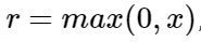
Then its gradient is:
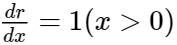
As the first layer is just the softmax function again its gradient is:
Where P is a vector of normalized probabilities. Finally this step also calls for backpropagation, which is just the application of the chain rule:
dscores = prob #softmax
dscores[xrange(N),y] -= 1 #gradient of softmax
dscores /= N

#backpropagating the gradient
grads['W2'] = np.dot(layer2.T, dscores) + reg * W2
grads['b2'] = np.sum(dscores, axis=0)

dscores1 = np.dot(dscores, W2.T) * (layer1>0)  #gradient of ReLU function

#backpropagating the gradient
grads['W1'] = np.dot(X.T, dscores1) + reg * W1
grads['b1'] = np.sum(dscores1, axis = 0)
Future Work
When I reached this part of the course the lecture videos were taken down. As it took me an incredible amount of time to do this assignment with the lecture videos, my teacher and I decided to focus on learning to work with deep learning libraries like torch as it will enable me to use deep learning for more practical applications. Here is a link to that repo. However, I have not given up on this course as I feel I still have a tremendous amount to learn from it!